


If you want to become a software engineer, but don’t know where to start, let’s save you the suspense: It’s algorithms and data structures.
Once you get the gist of these pillars of programming, you’ll start seeing them everywhere. And the more algorithms and data structures you learn, the more they’ll serve as jet fuel for your career as a software engineer.
To get you started, let’s first take a deep dive into Search and Sort, two classes of algorithms you can’t live without. Then let’s do a quick survey of the rest of the landscape that includes trees, graphs, dynamic programming and tons more.
Searching
Roughly speaking, there are two categories of search algorithms you’ll need to know right away: linear and binary. Depth First Search (DFS) and Breadth First Search (BFS) are also super-important, but we’ll save them for the graph traversal section below.
Linear search
The linear and binary algorithms are named as such to describe how long (time complexity) a search is going to take based on the size of the input that is being search.
For example, with linear search algorithms, if you have 100 items to search then the worst case scenario would require that you look at every item in the input before you came across your desired value. It is called linear because the time is takes to search is exactly correlated with the amount of items in the search (100 items/input =100 checks/complexity)
In short, linear = simple (there is nothing clever about the algorithm). For example: imagine you’re trying find your friend Lin among a line of people standing in no particular order. You already know what Lin looks like, so you simply have to look at each person, one by one, in sequence, until you recognize or fail to recognize Lin. That’s it. In doing so, you are following the linear search algorithm
Binary search
Binary search gets its name because the word binary means “of or relating to 2 things” and the algorithm works by splitting the input into two parts until it finds the item that is being searched. One half contains the search item and the other half doesn’t. The process continues until the spot where the input is split becomes the item that is being searched. Binary search is basically just a highly disciplined approach to the process of elimination. It’s faster than linear search, but it only works with ordered sequences.
An example should make this more clear. Suppose you’re trying to find your friend Bin (who is 5’5’’) in a single-file line of people that have been ordered by height from left to right, shortest to tallest. It’s a really long line, and you don’t have time to go one-by-one through the whole thing, comparing everyone’s height to Bin’s. What can you do
 Enter binary search. You select the person in the very middle of the line, and measure their height. They’re 5’7’’. So right away you know that this person, along with everyone to their right, is not Bin. Now that you’ve cut your problem in half, you turn your attention to the remainder of the line and pick the middle person again. They’re 5’4’’. So you can rule out that person and anyone to their left, cutting the problem in half again. And so on. After just five or six of these splits, you quickly home in on Bin in a fraction of the time it took you to find Lin. In doing so, you have followed the binary search algorithm.
Sorting
Ordering, otherwise know as sorting, lists of items is one of the most common programming tasks you’ll do as a developer. Here we look at two of the most useful sorting algorithms: MergeSort and QuickSort.
MergeSort
Let’s suppose that rather than coming across the ordered line of people in the example above, you need to create an ordered line of people out of an unordered group. You don’t have much time, so you come up with a strategy to speed things up.
You first have the group of people, which are all huddled together, divide into two. Then you have each of the two groups divide into two again, and so on, until you are dealing entirely with individuals. You then begin to pair the individuals up, and have the taller of the two in each pair stand to the right of the other one. Pretty soon everyone is organized into these left-right ordered pairs.
Next, you start merging the ordered pairs into ordered groups of four; then merging the ordered groups of four into ordered groups of eight; and so on. Finally, you find that you have a complete, height-ordered line of people, just like the one you encountered above. Without knowing it, you have followed the MergeSort algorithm to accomplish your feat.
QuickSort
QuickSort’s a bit too complex to easily picture with people, so let’s get a little closer to the code. To start, let’s imagine you have an unordered list, or array, of eight numbers that you want to order.
4 2 13 6 15 12 7 9
You could use MergeSort, but you hear that QuickSort is generally faster, so you decide to try it. Your first step is to choose a number in the list called the pivot. Choosing the right pivot number will make all the difference in how fast your QuickSort performs, and there are ready-made formulas to follow for choosing good pivots. But for now, let’s keep it simple and just go with the last number in the array for our pivot number: 9.
4 2 13 6 15 12 7 9
To make the next step easier to follow, we’ll create a separator at the beginning of the array and represent it with the pound-sign.
# 4 2 13 6 15 12 7 9
Moving from left to right through our array, our goal is to put any number smaller than the pivot (9) to the left of the separator, and any number greater than (or equal to) the pivot to the right of the separator. We start with the first number in our array: 4. To move it to the left of the separator, we just move the separator up one element:
4 # 2 13 6 15 12 7 9
We do the same with the next number: 2.
4 2 # 13 6 15 12 7 9
But then we get to 13, which is larger than the pivot number 9 and already to the right side of the separator. So we leave it alone. Next we come to 6, which needs to go to the left of the separator. So first, we swap it with 13 to get it into position:
4 2 # 6 13 15 12 7 9
Then we move the separator passed it:
4 2 6 # 13 15 12 7 9
Next up is 15, which is already to the right of the separator, so we leave it alone. Then we have 12. Same thing. But 7, our last number before reaching the pivot, needs the same kind of help moving as 6 did. So we swap 7 with 13 to get it into position:
4 2 6 # 7 15 12 13 9
Then, once again, we move the separator passed it:
4 2 6 7 # 15 12 13 9
Finally, we come to our pivot number: 9. Following the same logic as we have above, we swap 15 with 9 to get the pivot number where it needs to be:
4 2 6 7 # 9 12 13 15
Since all the numbers to the left of 9 are now smaller than 9, and all the numbers to the right of 9 are greater than 9, we’re done with our first cycle of QuickSort. Next, we’ll treat each set of four numbers on either side of the separator as a new array to apply QuickSort to. We’ll spare you the details, but the next round will give us four pairs of numbers to easily apply our final round of QuickSort to.
The end result will be the following ordered list that took us less time to generate than it would have with the simpler MergeSort:
2 4 6 7 9 12 13 15
Sorting algorithms cheat sheet
These are the most common sorting algorithms with some recommendations for when to use them. Internalize these! They are used everywhere!
Heap sort: When you don’t need a stable sort and you care more about worst case performance than average case performance. It’s guaranteed to be O(N log N), and uses O(1) auxiliary space, meaning that you won’t unexpectedly run out of heap or stack space on very large inputs.
Introsort: This is a quick sort that switches to a heap sort after a certain recursion depth to get around quick sort’s O(N²) worst case. It’s almost always better than a plain old quick sort, since you get the average case of a quick sort, with guaranteed O(N log N) performance. Probably the only reason to use a heap sort instead of this is in severely memory constrained systems where O(log N) stack space is practically significant.
Insertion sort: When N is guaranteed to be small, including as the base case of a quick sort or merge sort. While this is O(N²), it has a very small constant and is a stable sort.
Bubble sort, selection sort: When you’re doing something quick and dirty and for some reason you can’t just use the standard library’s sorting algorithm. The only advantage these have over insertion sort is being slightly easier to implement.
Quick sort: When you don’t need a stable sort and average case performance matters more than worst case performance. A quick sort is O(N log N) on average, O(N²) in the worst case. A good implementation uses O(log N) auxiliary storage in the form of stack space for recursion.
Merge sort: When you need a stable, O(N log N) sort, this is about your only option. The only downsides to it are that it uses O(N) auxiliary space and has a slightly larger constant than a quick sort. There are some in-place merge sorts, but AFAIK they are all either not stable or worse than O(N log N). Even the O(N log N) in place sorts have so much larger a constant than the plain old merge sort that they’re more theoretical curiosities than useful algorithms.
Non-comparison sorts: Under some fairly limited conditions it’s possible to break the O(N log N) barrier and sort in O(N)! Here are some cases where that’s worth a try:
Counting sort: When you are sorting integers with a limited range.
Radix sort: When log(N) is significantly larger than K, where K is the number of radix digits.
Bucket sort: When you can guarantee that your input is approximately uniformly distributed.
More must-have algorithms and data structures
Although Search and Sort are two of the most trusted, well-worn paths to take as you enter the world of algorithms and data structures, no survey of the landscape is complete without talking about the following favorites:
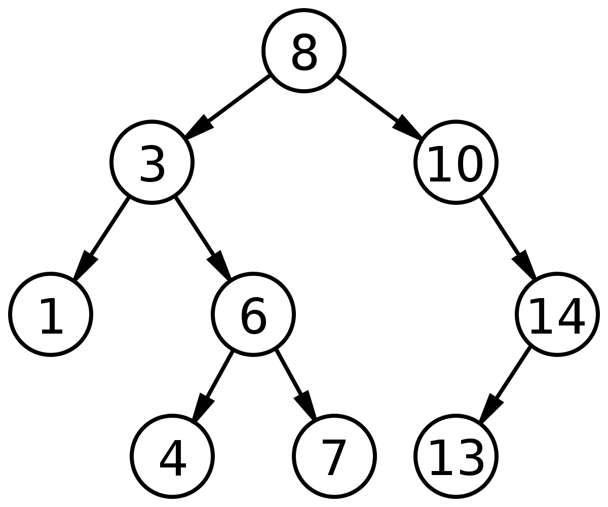
Trees
You’re going to see a lot of trees in your time, as they’re one of the most common data structures out there. They’re also one of the easiest data structures to picture and make sense of. Almost all of the terminology surrounding trees comes from the notion of a family tree. Depending on the position of a node (i.e. a family member) relative to other nodes in the tree, the node is called a parent, a child, a sibling, an ancestor, a descendant, etc.
Storing items in trees allows us to find items in a more efficient way if the tree has certain properties. (see Binary Search Tree below)
 Graphs
If you want to get technical, a tree is ultimately just a special case of a graph. So it’s no surprise that graphs are everywhere in daily life and computer science. In particular, graph traversal is a big deal, and there are two algorithms you’ll want to get a handle on quick: Breadth First Search (BFS) and Depth First Search (DFS).
To get a sense of what these two essential algorithms entail, imagine you’re at the top of a skyscraper shaped like a pyramid, and you need to search the whole building to find your friend Fiz. Then you realize that the pyramid is roughly equivalent to a graph where each room is a node.
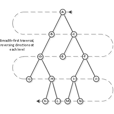
Breadth First Search (BFS)
If you traverse the pyramid floor by floor, starting with the top of the pyramid, you will be roughly performing a breadth-first search for your friend Fiz. Check out the visualization below to develop a better intuition about this type search and how it behaves.
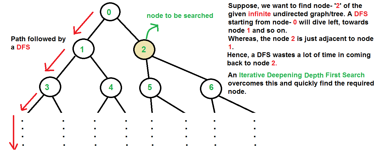
 Depth First Search (DFS)
Rather than going floor by floor, if you go elevator-by-elevator, checking the nearest rooms on each stop as you traverse the pyramid in vertical slices, you will be roughly performing a depth-first search for your friend Fiz. Again, the visualization below should help make this a bit more clear.
 Source: geeksforgeeks.com
Dynamic programming (DP)
If you’re facing an enormous, heavyweight programming problem that you can’t imagine solving on your own, Dynamic programming (DP) may come to your rescue. DP will help you turn the big problem into small sub-problems. Each time DP solves one of the sub-problems, it saves the results, and eventually puts all the results it’s saved together in order to tackle the big one.
Hashing
In recent years, there has been a sea change in how we find data. While the primary approach was once binary search, it’s now increasingly becoming the hash lookup. Although we’ll spare you the time-complexity comparison here, suffice it to say that when it comes to searching through lists with millions of items, hashing is often far faster.
String pattern matching
If you’ve heard of regular expressions (aka regex), you’ve already heard of string pattern matching. The idea here is that you’re not so much searching for an item, but a pattern that may be common to lots of items. For example, suppose you are searching a book for all sentences that end in a question mark: that’s a job for string pattern matching.
Still more…
We’ve covered a lot of ground. But we’ve still barely hinted at the grand scope of the world of algorithms and data structures. Here are a few more to sink your teeth into:
Data Structures:
Arrays
Linked lists
Stacks
Queues
Algorithms:
Primality testing
Fast Fourier transform
Binary exponentiation
Exponentiation by squaring
The road to software success is paved in algorithms
If nothing else, all of the above should pound home the idea that if you want to become a software engineer, algorithms and data structures will pave (and maybe even pay) the way for you. For a rock-solid foundation, you may want to start with Search (linear and binary) and Sort (SortMerge and QuickSort).
Once you get the gist of these pillars of programming, it’s time to learn everything you can about trees, graph traversal (BFS and DFS), dynamic programming and string pattern matching.
But the real goal is to start living and breathing algorithms and data structures: thinking up step-by-step solutions to real-world problems, and picturing complex scenarios in terms of simple data structures. If you can master that, then the coding will come naturally.
If you liked this post, I’ve got much more like it over at my personal blog (jasonroell.com).
Check it out and have a great day!